lab_4
Setting Ground Control Points (GCPs) and differential GPS correction (Post-processing Kinematic) for improved accuracy
Introduction:
Ground Control Points are very sensitive and very beneficial to land analyst who is trying to improve the accuracy of the survey. GCP is needed to get better quality of your analysis. For example, if you want to survey one particular site, and the site has very fluctuated weather conditions. Therefore ground on the site and its elevation would be alterable. We would probably need GCPs to obtain cm accuracy on the ground. Analysis with and without GCPs would be huge different. There are different kinds of GCP collecting methods.
 Figure 1. GCP collecting method.

Figure 2. GCP collecting method

Figure 3. GCP collecting method
As you can see from Figure 1,2 and 3, there would be different styles of collecting GCP data. However, I would highly recommend that getting a most precise center one like Figure 1.
To get "cm" accuracy for your survey, you would definitely need to have GNSS data, otherwise you might get above "m" accuracy. And this stands for Global Navigation Satellite System. There are 3 different formats that you can get GNSS data.

Figure 4. Study Area in Myrick Park, La Crosse WI.

Figure 5. Gun shelter that data was taken.
Myric Park is a 22 acre mostly wetland property within the La Crosse Area Comprehensive Fishery Area in La Crosse County. This large park connects to numerous trails, from easy to hard, featuring scenic views of the marsh and surround bluffs. The possible obstacles would be terrain formation on the ground. The terrain is declining from south toward north, therefore technically it is not a flat surface. Also trees could distract the flight mission. However, I would be fine if we just fly below 40 feet from the surface.

Figure 6. GPS logging and collecting GCP
Make sure you hold tightly and see the bubble eye that attached with rover and make the bubble locates at the center. This helps you hold and stand vertically correct. You also need to put rover on the exact center of the point.
The duration time was few second to maximum 60 seconds.

Figure 7. Wood stick to make pad stable.
After we have obtained the GCP data, we need to correct this data to be used in the data processing.
In order to get a "cm" accuracy, we would need "Differential Correction" As I mentioned previously, 'Differential Correction" we have received the base station file from the Wisconsin DOT website. The reason we had base station file, is the station data has been logging every seconds of the day. Therefore, we can applied this to our post processing.
There is a software called "GPS Pathfinder" that can correct our point data.
 Figure 8. Icon of GPS Pathfinder Office

Figure 9. Making Project folder
You first need to make a project folder that you would save your corrected point data otherwise, it will be very hard to tracking down your outcomes. First, name your file and import the base station file that you have downloaded from Wisconsin DOT.

Figure 10. Import the uncorrected points.
You now import the first GNSS file to be started.

Figure 11. Import Uncorrected points.

Figure 12. Correcting the point.

Figure 13. Result of the Point Correction.
As you can see, after we ran the correction, we have gotten 0-5cm accuracy point data.
Now we have to export as a shape file so we can open in the Arc map.

Figure 14. Exporting as a shapefile.

Figure 15. Set the projection and datum.
setup your path for output folder and change export file as shapefile and define your projection and datum that you would use.

You need to check the attributes that should be shown on the Arc MAP.
After export your first GNSS point, you have to do the same processes for the 2nd GNSS, Therefore, we will merge in the Arc map by using Merge tool.
Let's go to Arc map.
 Figure 17. Arc map.

Figure 18. Merge tool
In the Arc Map software, we can merge the corrected points from the GPS Pathfinder.
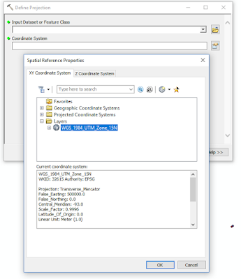
Figure 19. Define the projection and datum in Arc Map.
After you have merged, you need to define the projection and datum. In this case, WGS_1984_UTM_Zone_15N.

Figure 20. Export attribute table as an csv file.
In csv file, we need to compile the table. You would need to remove the attribute except Northing, Easting and GNSS height.

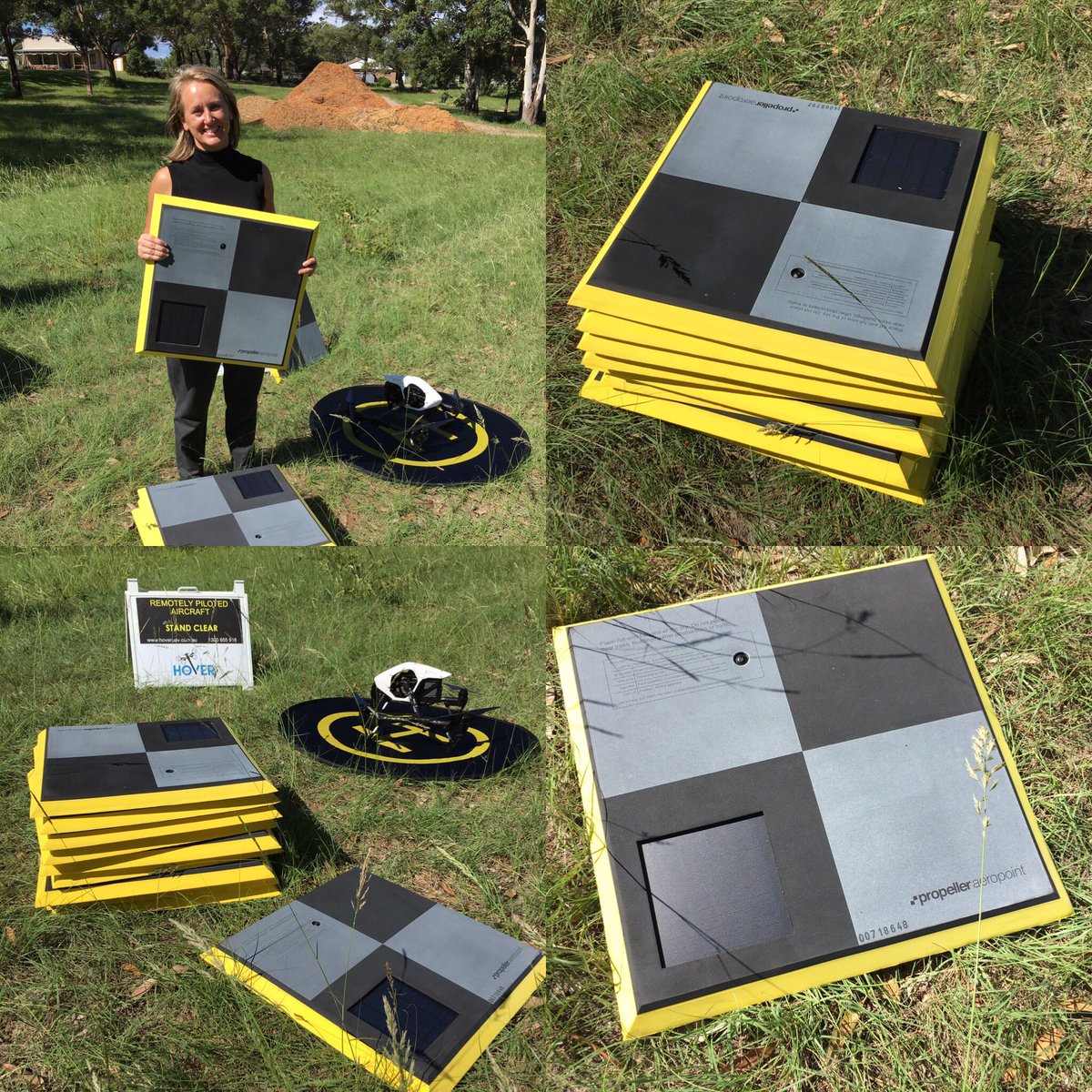

Figure 2. GCP collecting method

Figure 3. GCP collecting method
As you can see from Figure 1,2 and 3, there would be different styles of collecting GCP data. However, I would highly recommend that getting a most precise center one like Figure 1.
To get "cm" accuracy for your survey, you would definitely need to have GNSS data, otherwise you might get above "m" accuracy. And this stands for Global Navigation Satellite System. There are 3 different formats that you can get GNSS data.
Real time correction:
This is also called RTK. The rover that you hold on top of the GCP site, it is basically perceived the data from the base station by internet connection. It is not a best way to collect the GNSS data because your have and body is not fixed.
Differential GPS (DGPS):
This would be the better than RTK because, it uses fixed and known position to improve the error form the RTK.
SBASS:
In United States, we use WAAS(Wide Area Augmentation System). There are other types of SBASS over the world. EGNOS(Europe), GAGAN(India) and MSAS(East Asia). The data are collected by geostationary satellites. Therefore we expect to receive high accuracy.Study Area:


Figure 5. Gun shelter that data was taken.
Myric Park is a 22 acre mostly wetland property within the La Crosse Area Comprehensive Fishery Area in La Crosse County. This large park connects to numerous trails, from easy to hard, featuring scenic views of the marsh and surround bluffs. The possible obstacles would be terrain formation on the ground. The terrain is declining from south toward north, therefore technically it is not a flat surface. Also trees could distract the flight mission. However, I would be fine if we just fly below 40 feet from the surface.
Methodology:
In our lab, we have made 8 GCPs that are widely and equally distributed so we can get data from everywhere. We grouped together and brought GNSS rover to collect the GCP data. The projection and datum we had used were UTM Zone 15N and WGS 1984.

Figure 6. GPS logging and collecting GCP
Make sure you hold tightly and see the bubble eye that attached with rover and make the bubble locates at the center. This helps you hold and stand vertically correct. You also need to put rover on the exact center of the point.
The duration time was few second to maximum 60 seconds.

Figure 7. Wood stick to make pad stable.
After we have obtained the GCP data, we need to correct this data to be used in the data processing.
In order to get a "cm" accuracy, we would need "Differential Correction" As I mentioned previously, 'Differential Correction" we have received the base station file from the Wisconsin DOT website. The reason we had base station file, is the station data has been logging every seconds of the day. Therefore, we can applied this to our post processing.
There is a software called "GPS Pathfinder" that can correct our point data.


Figure 9. Making Project folder
You first need to make a project folder that you would save your corrected point data otherwise, it will be very hard to tracking down your outcomes. First, name your file and import the base station file that you have downloaded from Wisconsin DOT.

Figure 10. Import the uncorrected points.
You now import the first GNSS file to be started.

Figure 11. Import Uncorrected points.

Figure 12. Correcting the point.

Figure 13. Result of the Point Correction.
As you can see, after we ran the correction, we have gotten 0-5cm accuracy point data.
Now we have to export as a shape file so we can open in the Arc map.

Figure 14. Exporting as a shapefile.

Figure 15. Set the projection and datum.
setup your path for output folder and change export file as shapefile and define your projection and datum that you would use.
Make sure your unit for the coordinate is centimeters because, now our data is centimeter accuracy.

Figure 16. Set the attributes
You need to check the attributes that should be shown on the Arc MAP.
Let's go to Arc map.


Figure 18. Merge tool
In the Arc Map software, we can merge the corrected points from the GPS Pathfinder.
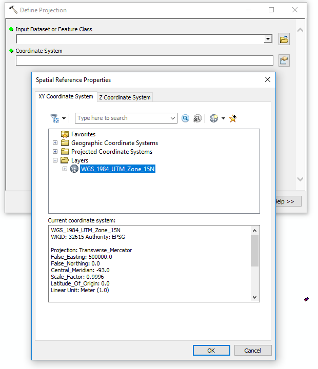
Figure 19. Define the projection and datum in Arc Map.
After you have merged, you need to define the projection and datum. In this case, WGS_1984_UTM_Zone_15N.

Figure 20. Export attribute table as an csv file.
In csv file, we need to compile the table. You would need to remove the attribute except Northing, Easting and GNSS height.
Results:
This kind of process will help researchers to have good quality of the project outcome. We were able to obtain 0-5cm accuracy which is very accurate, moreover, the accuracy can be more improved by logging longer time. The correction process has been taken about 10 minute.

Figure 21. Points that were corrected and uncorrected on the mosaic image.
Discussion:
In out lab, we exported both uncorrected and corrected points to compare the location on the actual mosaic image. Apparently, we can see the little moves between corrected and uncorrected points. Therefore, we can prove that with and without using GCP is influential. You would get much better accuracy on your image location but like we did, you need to spend the extra time to get it.Conclusion:
Now so far, we did great job to get a 0-5cm accuracy and we have learned that how much important having a GCP point and how this can effect our quality of project. For next lab, we would use this data in the Pix4D mapper and see what might be the difference from the previous processing.
Comments
Post a Comment